|
|
|
|
|
||
| Home | ||
| Tutorial | ||
| Case Study | ||
|
|
Manual | |
| Data | ||
| General Info | ||
| Template Matching | ||
| Aligning Datasets | ||
| DTW algorithm | ||
| Thanks | ||
| Download | ||
| Tutorial | |||
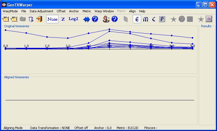
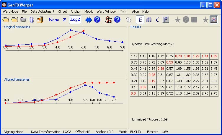
Aligning Session As the name suggests, the aligning datasets mode allows finding the best time alignment between two sets of gene expression time series and it can be useful for comparative studies of the temporal behaviour of a set of genes in different experimental conditions (e.g. cell cycle expression data generated with different synchronization techniques) or in different organisms (yeast, plants, human, etc.). The two profile sets are supplied separately in two different files. The files are supposed to have the same number of profiles and the corresponding profiles must appear respectively in the same order in both files. The aligned suite can be saved into a file, which may consequently be subjected to further studies with other microarray analysis tools. In the example below, the time expression profiles of all CYCB genes from the aphidicolin addition synchronization experiment of Menges et al., 2003(1) (Data) have been loaded into GenTχWarper.
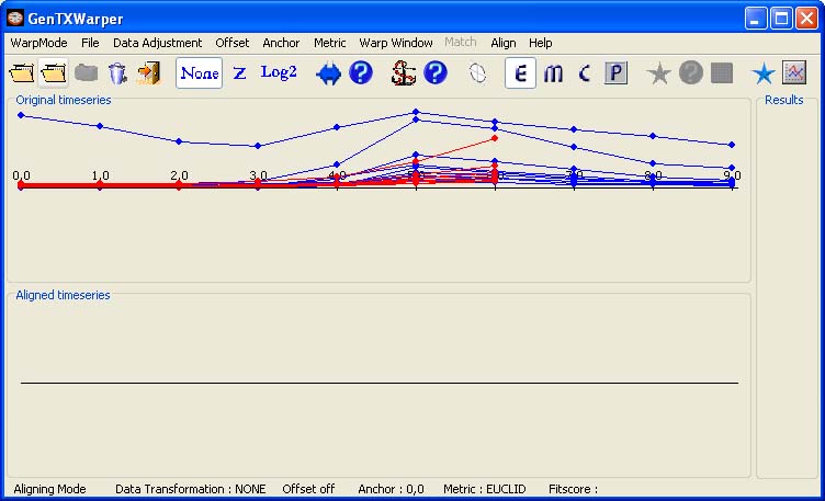
Next, the time expression profiles of all CYCB genes from the sucrose starvation synchronization experiment of Menges et al., 2003(1) (Data) are loaded and displayed in red.
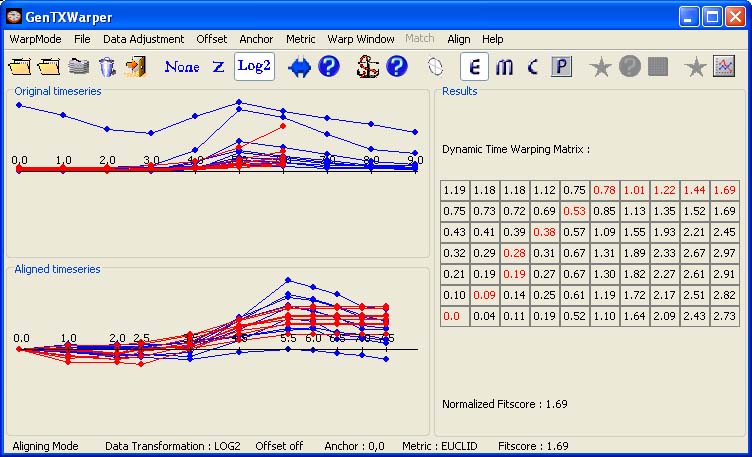
The two sets of expression profiles have been generated in different experimental conditions and consequently, the comparison of their absolute expression values will not be very meaningful. Therefore before proceeding with aligning the two sets of profiles it is better to transform them to relative expression values by aplying log2-transformation (Data). Then the two time series can be aligned by simply selecting Align! in the Align menu. Alternatively, the following tool bar button can be used:
The two visualization panels provide a comparative view of 1) the original expression profiles (top panel); 2) their aligned with the DTW algorithm counterparts (bottom panel). Additionally, GenTχWarper reports in the right window the DTW matrix with the optimal warping path through it indicated in red, and the final fitscore after normalization.
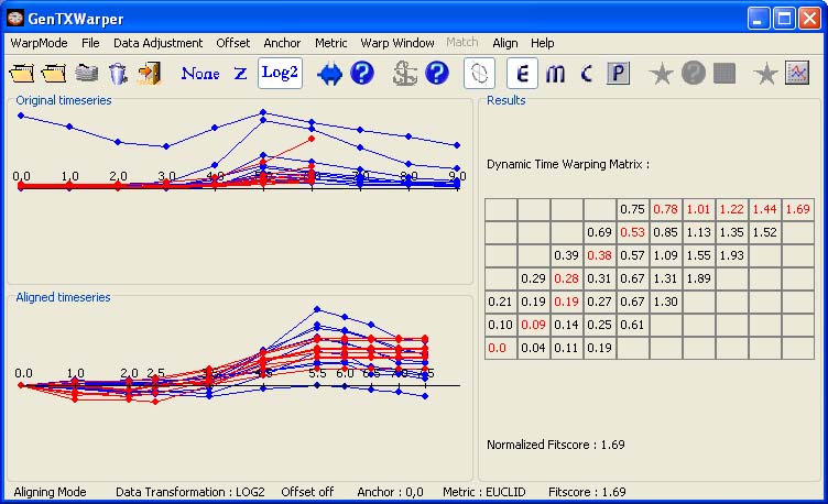
Applying a Warping Window The alignment of large sets of time series may be rather time consuming. The warping window constraint allows to reduce the search space and consequently speed up processing of large microarray data sets. The effect of the application of a warping window of size 3 on the calculation of the DTW matrix can be witnessed in the figure below.
Average View The visualization of the
comparison of large sets of gene profiles will
not be very informative due to the presence of large number
of aligned individual profiles which will be
plotted on top of each other. One can choose for visualization of
average profiles, instead. The latter feature of the alignment mode can be selected from the
Align menu by clicking on Average
View, or via the tool bar button:
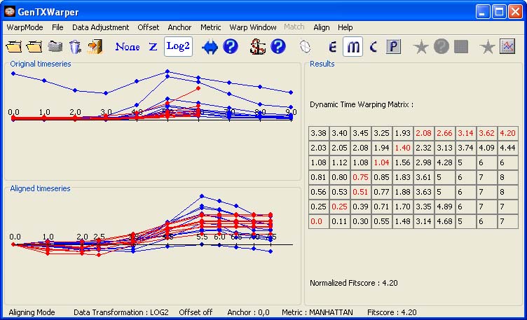
Choosing a Distance Measure The optimal alignment above is resulting from minimizing the total distance between the two sets of expression profiles when the distance between each pair of matching time vectors is estimated using the Euclidean distance. Presently, two other distance metrics between the time vectors can be used within GenTχWarper: Manhattan and Chebychev. The particular choice of a distance metric will affect the resulting alignment. 1) The Manhattan distance is just the sum of the absolute values of the differences between the corresponding vector dimensions. In comparison to the Euclidean distance, it tends to yield a larger numerial value for the the same relative position of the points. This is illustrated below with the alignment of the same CYCB's as above, but when the Manhattan distance is applied.
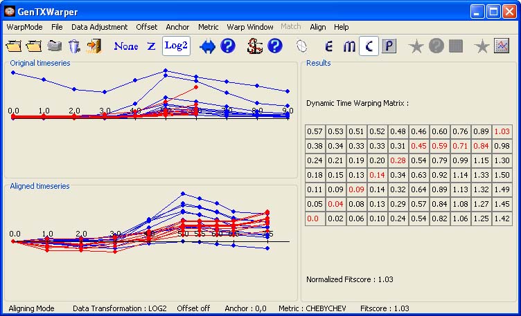
2) The Chebychev distance will simply pick the largest difference between any two corresponding time points and consequently, it should be used when the goal is to reflect any such big difference. One has to keep in mind however, that the Chebychev distance behaves inconsistently with respect to outliers since it only looks at one dimension. The alignment of the CYCB's profiles when the Chebychev metric has been used to calculate the distance between each pair of time vectors is given below. It differs from the alignments obtained with the Euclidean and Manhattan metrics above.
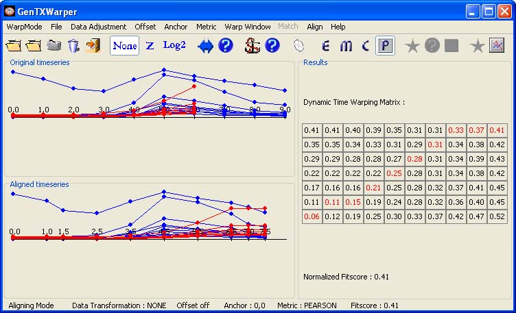
3) The Pearson correlation distance is supposed to measure the similarity in shape between two vectors. The formula for the Pearson correlation distance is: d = 1 - r where r = Z(x) · Z(y) / n is the dot product of the z-transformed values of the vectors x and y. If the two vectors compared represent the sets of expression values of given genes in a particular time point for two different experiments respectively, then r will be high if the genes vary in a similar way in the two experiments even if the magnitude of change differs a lot. The CYCB's profiles have been aligned below by calculating the Pearson correlation distance between each pair of time vectors.
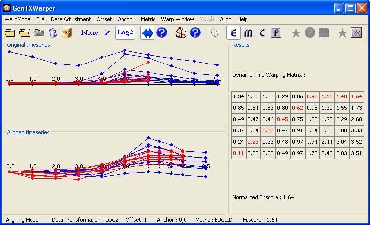
Applying an Offset The offset function enables sliding the time series against each other along the time axis (General Info). In the context of the aligning datasets mode, applying an offset can be useful in the following cases: 1) Many biological processes, as for instance cell cycle, are conserved between species, and for a given gene with a known function in one species, one may attempt to identify a set of genes in another species with a potentially similar function. However the duration of the different cell cycle phases may vary considerably between species and one way to correct for this is to apply an offset, eventually in a combination with an anchor point (see below), that positions the corresponding cell cycle phases of interest against each other. Otherwise one risks to identify many genes that pick more or less at the same time, relative to time zero, as the template gene, but in completely different cell cycle phase. 2) The possibility for applying an offset is also essential in case the biological process under study displays a phase shift due to the design of the experiment. For instance, cell cycle progression is usually studied via genome-wide expression profiling of synchronized cell suspensions cultures and usually different methods will generate a synchronized resumption of different phases of the cell cycle. The later is actually true for the two synchronization methods, aphidicolin addition and sucrose starvation, used by Menges et al., 2003(1) (Data). The former method generates a synchronized resumption of the S-phase, and the latter results in a synchronized transition from G1 to S. The best alignment (a diagonal path) between the profiles of the CYCB genes from the two different experiments has been obtained, as shown below, for an offset 1 corresponding to 2 hours. The blue profiles have been shifted with 1 time point to the right of time zero. Thus the phase shift between the aphidicolin addition and the sucrose starvation synchronization for the CYCB genes seems to be about 2 hours.
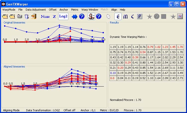
Using an Anchor Point The anchor point option provides the possibility to explicitly align a time point from one time series with a time point from another time series and can be used in similar cases as the ones listed above for the offset. For instance, the alignment of the two CYCB time series presented below is obtained after setting an anchor point (0,1), marked in blue in the DTW matrix. The result is very similar to the one with an offset 1 above. The difference is that the alignment is performed over the whole time interval, while in case of an offset 1 only over the interval [1,8].
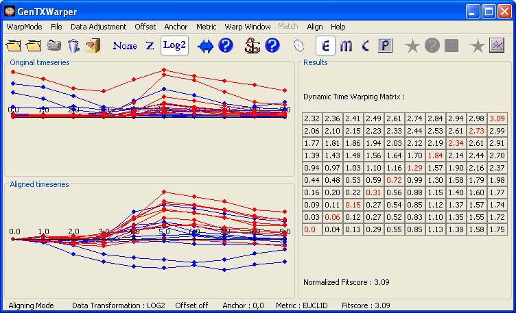
Within Experiment Alignment The alignment mode can also be used to compare the time trajectories of two groups of genes of interest coming from the same time series data. In the example below, the time expression profiles of the CYCA (in blue) and CYCB (in red) genes coming from the aphidicolin addition synchronization experiment (Data) are aligned against each other. The perfect match (a diagonal optimal alignment path) indicates that as groups CYCA and CYCB have very comparable behaviour during the aphidicolin addition synchronization.
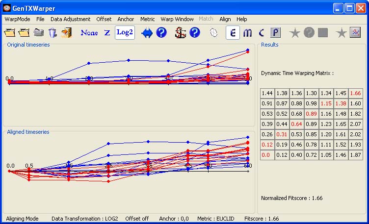
This is not the case for the sucrose starvation synchronization (Data) however, as illustrated in the figure below. The expression profiles of the CYCBs (in red) show a certain delay with respect to the CYCAs (in blue) at the beginning of the synchronization, most probably due to some stress response effects.
(1) Menges,M., Henning,L., Gruissem,W., Murray,A.H. Genome-wide gene expression in an Arabidopsis cell suspension. Plant Molecular Biology, 53, 423-442 (2003).
|
|