In the following sections, we specify each statement (=recognized command) of the simulator. We will represent them as "regular expressions".

Regular expressions are commonly used to define the syntax of a line of text. They tell what is allowed so that the simulator will understand a command. They usually are a keyword (the command), followed by a number of optional arguments (=extra information).

A regular expression describes the real command as follows:
  - 'text' means the literal text as it is typed between the quotes;
  - <text> means a number or a string that you can freely choose  (a string is
                 a sequence of letters/numbers/characters, starting with a letter);
  - [abc] is zero or one occurences of abc;
  - (abc)* is zero or more occurences of abc;
  - (abc)+ is one or more occurences of abc;
  - ( a | b ) means either a or b;
  - text  (italic font) will be a pointer to another regular expression.

For example, the regular expression  ( 'bla' | 'a' )*  would allow the text  blabla  and  ablaablaaaa  , but not  blabl  .

Now we will give each statement's syntax along with a few examples, and explain it a bit more detailed, in the following way:
 

 

comp

'comp' <name>  [<initialAmount> [<degradationRate>] ]                                                                                                                                 [colorDef | 'noplot']     colorDef   <colorname>     |     '('  <redValue0to255>  [',']  <green>  [',']  <blue>  ')'    red green light_blue (255, 0, 0) (255  255  0) (128  128  255)   comp  CDC25 comp  CDC25  100 comp  CDC25  100  0.05   comp  CDC25   red comp  CDC25  100  red comp  CDC25  100  0.05  red comp  CDC25  100  0.05  (255, 0, 0)

All components (mRNA or proteins) you wish to use in a simulation must first be defined with the comp statement. This statement can have up to four arguments: the component's name, an initial amount, a degradation rate, and a color.

The component's initial amount is how much component there is at the start-time defined with the starttime command. If you don't explicitly define starttime, the simulator will use the default value for the start time, which is "time = 0".

The optional degradation rate (which must always be given as the third argument) reflects natural break-down by proteases, nucleases etc.  For example a degradation rate of 0.05 would destroy 5% of the present component per time unit.
Note that component units and time units are arbitrary. These can be numbers of molecules, moles, seconds, days etc.

As a last argument, you can give a color. If you do this the component will also be plotted in the combined view window of SIM-plex, in the requested color. If you don't give this color argument then the component won't appear in the combined view but will only be plotted in the separate-views-window.
You can give a colorname from the X11 list, or define it by its red, green and blue values (0=no color, 255=maximum of that color), for example (255,0,0) is pure intense red.
Instead of a color, you can type noplot. This will make the plot dissappear from the Combined Plot as well as from the Single Plot window. This is useful when you want to focus on other components.

 

virtcomp

'virtcomp'  <name>  =    [<factor> ['*'] ] <compName>                                                                ( '+'  [<factor> ['*'] ]  <compName> )*                                                 [colorDef | 'noplot']                                                                            virtcomp V = A + B virtcomp V = 0.5 A + 0.8 B virtcomp V = 0.5*A + 0.8*B virtcomp V = 0.5*X + 0.8*Y + C virtcomp V = A + B   red virtcomp V = 0.5 A + 0.8 B  red virtcomp V = 0.5*A + 0.8*B   red virtcomp V = 0.5*X + 0.8*Y + C   red

The concept of a virtual component allows the simulator to deal with problems like the following: if a protein A is produced, and at the same time B is produced  through a different process (for example, it's a less active derivative of A), and A and B have an additive effect on the regulation of C. How would you express this in statements like "if ...>... then ..."? You would need something like "if  (...+...) > ...  then ...". To avoid additional complexity in the if-then definitions, we allowed defining virtual components. In the example, the virtual component V is defined as "A + 0.5 * B", and this virtual V subsequently is the regulator of C.

To be able to handle this feature, the mathematics of Piecewise Linear Differential Equations (PLDE) needed to be extended a little in SIM-plex. Next to the piecewise linear differential equations, when defining virtual components, also linear combinations of PLDEs are used.

Note: you cannot define a virtual component in recursive terms or with component names that are not yet defined.

 

fixedcomp

'fixedcomp'  <name>                                                                                                                    [ 'repeat' ]   <timepoint>  <compAmount>                                                       ( ','  [ 'repeat' ]   ['add']  <timepoint>  <compAmount>  )*                             [ colorDef  |  'noplot' ]                                                                              (Note: only one occurence of 'repeat' is allowed )                                               fixedcomp  comp1   0  0,  11  0,  13  10,  15  0,  31  0,  33  10,  35  0   blue fixedcomp  comp2   0  0,  add 11  0,  add 2  10,  add 2  -10,  add 5  0,                                             add 11  0,  add 2  10,  add 2  -10,  add 5  0 fixedcomp  comp3   repeat  0  0,  add 11  0,  add 2  10,  add 2  -10,  add 5  0

A fixed component represents a pre-defined course of a component's amount through time. It can be used if you have measured quantitative data for one component, and you want to see how hypothetically dependent other components react.

The three examples clarify how the fixedcomp statement works.
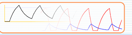
 - The example with 'comp1' is the simplest: it defines a sequence of timepoint+componentamount couples separated by comma's. If you try it out in SIM-plex, you will see a profile with two peaks.
 - The example of 'comp2' (two lines long!) defines the exact same profile as for 'comp1', but now uses the add keyword, that adds a time+amount to the last co-ordinates. This is useful because it makes a profile a lot easier to change. And in the example you could e.g. use copy-paste to quickly add another peak.
 - The example of 'comp3' uses the repeat keyword to define an infinite number of peaks like the two peaks in the 'comp1' and 'comp2' profile. Note that the repeat keyword can occur anywhere between the co-ordinates (though only once). This way you can first define a start-profile, which is then repeatedly followed by the sequence after the 'repeat' keyword. Note that the first component amount defined in the repeat tail should be equal to the last amount, to allow the repeats to link up.

 

2.  Conditional processes:  if ... then

 

if ... then ...

'if'  condition  ('and' condition)*   'then'  <compName>  <creationRate>      condition    'true'     |     (  <compName> ( '<' | '>' | '>=' )  (<threshold>)  )   true (This is the way to define "always", or "constitutively expressed") Rum1 < 40 (means: "if the Rum1 geneproduct is below the threshold of 40") Cdc25  >  50 (means: "if the Cdc25 geneproduct is above 50 units") if  true  then  MPF  5                (MPF could be the "mitotis-promoting factor" complex) if  Cdc25 > 50  then  MPF  5 if  Cdc25 > 50  and  Rum1 < 40   then  MPF  5

Biology, mathematics and the interface

If-then statements are at the heart of the simulator's interface. They formulate what happens in a genetic regulatory network, in a stepwise way. They approximate gene-activation or repression in a step-wise manner, as if it happened with switches, but then allowing the possibility to include more than one step between the "on" and the "off" state.

Gene regulation may happen by several proteins that bind to a gene's promotor sequence, together controlling how active the gene is expressed. Generally, the relation that describes a gene's (de/)activation in function of a regulatory protein's concentration, usually is sigmoidal (the mathematical function has a sigmoidal shape⁽¹⁾.).  In the Piecewise Linear Differential Equations (PLDE) model, these sigmoids are approximated by step functions. In case of activation, this means that as long as the regulatory protein's concentration stays below a certain threshold, the gene is in "off" state, and as soon as the regulatory protein reaches the threshold or rises above it, the gene is in "on" state. This is an approximation but Glass and Kaufmann showed⁽¹⁾ that a biological switching network that is approximated in this way, can have the same outcome as the original network.

The SIM-plex simulator is built on the PLDE model, and offers a very user-friendly interface that lets the user define these kinds of regulation without being bothered much by the underlying mathematics. The goal of the interface is to let the user work at a level above the mathematical equations, 'closer' to biology. When a simulation is executed, there first is a translation of the user's statements to mathematical equations. This translation can happen very transparent because there is an exact relation between the user's if-then statements and the stepwise activation functions that the PLDE model uses.

The if-then statement

Most genes are active only under certain conditions. For example: only if protein A is present in sufficient abundance, and protein B is virtually absent, the transcription of C is activated. This condition and the resulting gene-activation can be formulated in SIM-plex as "if  A > 20  and  B < 5  then  C  3".

You can see that after the if keyword, you can build a condition that is a chain of simpler conditions that are separated by the and keyword. A simple condition always compares the available amount of one component to a certain threshold. After the then keyword, you can give a component's name and the rate at which this component should be created when the all of the defined conditions are met.

Knowing an exact value for a threshold would of course be the ideal case, but with the current status of biological knowledge we often only know relative values, like "This component is very abundant. Some other component is less abundant. And some are not present at all at some timepoint."  Therefore it is not crucial - at this point in time - to use exact values. Estimates are good enough. As long as you see that the network you defined is able to show the expected behaviour with a given set of parameters, it is a good indicator that you know most of your network's components. If not, then you can start introducing hypothetical components and see if the simulator is able to predict functionality for this new network. In this way SIM-plex can be a useful tool for hypothesis generation.

Additivity

It happens a lot that gene activation changes as soon as an additional protein comes along to bind to the promotor. To facilitate the definition of such events, the if-then statements in SIM-plex were designed to work additively.
At each point in time, all statements that create a component P under a condition 'true' are summed together.
Take the example from the tutorial:
     if  A > 20  then  B  3
     if  B > 20  then  B  2
In this example, when A rises above 20, B is activated and created at a rate of 3. After that, when B rises above 20, B enhances its own transcription, by creating an additional 2 component-units per time-unit. From then onward, the creation rate of B increases to (3 + 2 =) 5.

Notes

1. In any if-then statement, also in the variants that follow below, you can also give threshold values and creation-rates by means of the name of a user-defined constant (see below how to define constants).
2. Keep in mind that there is a difference in meaning between positive and negative creation rates. It was explained in the tutorial, and will be repeated shortly (under the explanation of the if ... then ... block statement).
3. Component units and time units are arbitrary. These can be numbers of molecules, concentrations, seconds, days etc.
4. The underlying mathematical model works with half-open intervals. Every border between two intervals (divided by a (de/)activation threshold), always belongs to the upper interval. For example if the real numbers are divided by two thresholds, 4 and 8, then there will be piecewise-linear-differential-equations defined over each of the three intervals: [0, 4[  and  [4, 8[  and  [8, +∞[.  That is why conditions are only built with the comparators <, >, and >=.  (Note that >= means ≥).  ( > will have the same mathematical translation as >=. It was only made available for who wants to type it absolutely correct).
   Note that  [a, b[  means "everything between a and b, a inclusive, b exclusive".
5. Because of Note 4, the special condition "X > 0" will always yield "true" (because > equals >=, and the first halfopen interval is [0, firstThreshold[. 
   Because we still wanted it to be possible to make a distinction between quasi-zero and more than this 'quasi-zero', we addressed this problem by making SIM-plex translate any condition "X > 0"  to "X > lowNonZeroThreshold". This lowNonZeroThreshold is a very low threshold that has a default but adjustable value in SIM-plex (see below, under the default section).

 

if ... then ... block ...

'if'  condition  ('and' condition)*   'then'  <compName>                               'block'  [  ( <blockFactor0to1>  |  <additiveNegativeBlock> )  ]   if  Rum1 > 40   then  MPF  block               (complete block) if  Rum1 > 40   then  MPF  block  0.15     (partial block, 15% gets through) if  Rum1 > 40   then  MPF  block  -5         (partial block, subtracts 5 units / timeunit)

Even when sufficient transcription activating proteins are binding to its promotor, a gene can be partly or completely deactived if an inhibitor protein gets a grip on the promotor too, thereby interfering with the recruiting of the transcription machinery. This is what a block tail in an if-then statement can model.

There are three ways to use the if-then-block statement:

-  "... then  X  block"	(without an extra argument): this will completely block all creation of X, described by all other if-then statements.
-  "... then  X  block  addition"	(with a negative addition): this subtracts a value from the original creation rate, but cannot make it lower than zero.
-  "... then  X  block  factor"	(with a factor between 0 and 1):  multiplies the creation rate (áfter possible negative additions), with the given factor. For example "block 0.15" would restrict the creation rate to 15% of its original value.

To dertermine the type of block (multiplicative or subtractive), SIM-plex makes a simple distinction based on the value that follows the "block" keyword:
   - if it is between 0 and 1, it's interpreted as a multiplicative block;
   - if it is < 0, it's interpreted as an additive block. (Adds a negative rate).

A few examples:
   block 0.9  lets 90% of the transcription go on;
   block 0    blocks everything, just like "block" without argument;
   block -2   subtracts 2  (or "adds -2", hence "additive block") units per time-unit.

Note: in order to completely block the transcription of a network component, the only valid way is with these "block" statements. This will prevent context-dependency, like using +5, and -5 to get back to 0: the +5 could for example become a +8 at some time. Thus using "block" is the effective way to be sure that creation really stops.

Naturally, the "block" statement cuts off transcription-product creation rates to 0 when additive blocks sum together to a negative rate. While additive blocks are only meant as extra functionality, we believe that multiplicative blocks (with a factor) will be used in most cases.

 

if ... then ... nonreg ...

'if'  condition  ('and' condition)*   'then'  <compName>                                     'nonreg'  <creationRate>                                                                            if  Cdc25p > 40   then  MPF  nonreg  2.5

The difference between   "... then A 5"   and   "... then A nonreg 5"   is that the former models transcriptional creation which can be regulated by block statements, and the latter, "nonreg"-creation, can not be regulated by blocks.

To explain this, assume that one simulates supposing that mRNA is very quickly translated to proteins, and only a single "geneproduct" is used (instead of two, mRNA and protein).  When some biochemical operation happens so that the protein is produced (e.g. dephosphorylation of its phosphorylated counterpart), then this biochemical production part can not be affected by blocks, while the transcription part can still be under a "block" at the same time.
Instead of using the "nonreg" tail it is preferred to use the more powerful if-then-transform statement, which is described below and it makes use of the nonreg-functionality.

Note that "nonreg" followed by a negative rate has the same effect as when the "nonreg" would be omitted (e.g. "A nonreg  -5"  and  "A  -5"), because break-down always has a not-transcriptional cause, and can not be regulated by "block" statements.

 

if ... then  transform ...

'if'  condition  ('and' condition)*   'then'                                                      'transform' (<sourceName> |    '('  (<sourceName>)+  ')'    )           'to'               (<targetName>    |    '('  (<targetName>  )+  ')'    )           <rate> [<lowestThreshold>]                                                           if  A > 40  then  transform  B  to  Bphosph  2.5 if  true  then  transform  (A B)  to  C  2 if  true  then  transform  (A A B)  to  C  2 if  true  then  transform  (A B)  to  (C D)  2 if  true  then  transform  (A B)  to  (C D)  2  0.001

The section above shows an if-then statement with a transform clause in its tail, which is actually a shorthand for:
   "under the given conditions, break-down the source component", and
   "under the given conditions, create the target component at the same rate".
Thus the transform clause effectively specifies the two commands together. Prior to simulating the interactions, this if-then-transform statement is translated into two (or more) normal if-then statements like the above.
→ Note that special care had to be taken to let the creation of the target stop as soon as the source is depleted. Therefore the condition of the original transform statement is extended during the translation to plain if-then statements, by adding the condition "and sourceComponent > 0".
But this special condition gives problems with the mathematical model that is used!
As explained under the plain if-then statement's "Note 5" and "Note 4", the integration interval will be the half-open interval [0, firstThreshold[ . As this condition is always true (since >0 is also translated as >=0, see also Note 4), this extra condition had to be changed into "and sourceComponent > lowNonZeroThreshold". This lowNonZeroThreshold is a very low default threshold that is adjustable in SIM-plex (see below, under the default section). It can also be given as an additional argument to the transform statement.
The following example shows how this translation happens:
   "if  A>40  then  transform  X  to  Y  5"
is translated to the following two statements:
   "if  A>40  and  X > lowNonZeroThreshold   then   nonreg   X  -5"
   "if  A>40  and  X > lowNonZeroThreshold   then   nonreg   Y  5"
Note that "nonreg" is used because biochemical transformation cannot regulated by block-statements, as described before.

More general, an if-then-transform statement could be used to model the binding of proteins, or the splitting of a component, or for catalysing many to many. The "to" makes the distinction between the "source" and "sink" side, and if one side contains more than one component, it must be enclosed between brackets.  Note that when a reaction would need one A and two B's to form C, then you could define: "if ... then transform (A B B) to C  <rate>".

 --- We are aware that these not-regulatory biochemical operations are quantitatively less correct in the mathematical framework we use (i.e. linear creation/consumption and exponential degradation).  But in a genetic network that is already a quantitative approximation of reality, we deem that this method can still provide a very useable functionality to complete the definition of these switch-like networks ---

Note: you really should define a protein and its phosphorylated form as two different components, because they are two different biochemical entities too, which can be transformed into one another.

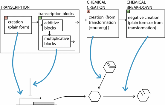
Note about creation, block and break-down

The if-then statement can have different tails, with different meanings. These were already described above. Here is an overview:

(1) and (2) model transcriptional creation, regulable by "block" statements, while (3) and (4) model (non-regulable) biochemical creation and break-down.
Note that in (4), you could also add "nonreg", but the negative rate already shows that it models biochemical breakdown, so it's not really necessary to tell this twice.

The following figure illustrates the sequence of calculations that determines the final creation rate or break-down rate in SIM-plex, in the most complicated case:

 

timepoints

'timepoints'  oneTimepoints_def  ( ',' oneTimepoints_def)*                           oneTimepoints_def   <timepoint>  |                                                                                                         <beginTime> 'to' <endTime>  [ 'step' <stepsize> | 'steps' <nrofsteps> ] 2 0 to 100 0 to 100 step 0.1 0 to 100 steps 1000 timepoints   0 to 100 timepoints   0 to 200 step 0.1 timepoints   0 to 100 steps 1000,  100 to 200 step 0.1,  201,  202,  203 timepoints   200 to 300

With this command you can tell the simulator for which timepoints you want to see the state of the simulated network. You can give it in a list separated by comma's, and most easily with the "step" or "steps" clause.
For example,   "timepoints 0 to 10 steps 100"   specifies that you want 100 small steps between 0 and 10.  Consequently, you will get the simulation result for the 101 timepoints:  0,  0.1,  0.2,  ...,  9.9,  10.
The command   "timepoints 0 to 10 step 0.1"   tells that you want to make steps of size 0.1, also resulting in the 101 time points  0,  0.1,  0.2,  ...,  9.9,  10.

If no stepsize or number-of-steps is given, a default number-of-steps is used: see below at the default statement.

The more timepoints you request, the more detailed the simulation plots will be. This command is also useful if you only need certain fixed timepoints, for example when you work with the command-line interface.

 

starttime

'starttime'  <time>                                                                                                 starttime 0 starttime 100

This statement determines at what time the simulation starts. This is the time at which all the components have their 'initial amounts'.  It is not necessarily the first timepoint for which results will be plotted: that should be done with the timepoints statement.

SIM-plex will report an error if the first requested time point comes before this starttime, because backward simulation is not possible.

 

const

'const'   <name> '=' value   ( ',' <name '=' value )*                                        const  MPFthreshold = 30 const  MPFthreshold = 30,  Rum1_thr = 40

With this command you define constant values that you can use for example for thresholds and rates in if-then statements.

 

sim

'sim'   (  'bruteforce';   <timestep>   |   ...  )                                                       sim  bruteforce  0.001 sim  bruteforce  0.005

This command is intended to allow you to select which simulator you want to use and what options you select for it.

Currently, however, only a "bruteforce" simulator has been implemented. It performs the simulation in small timesteps. At each timepoint, the creation/break-down rate of each defined component is calculated, and a small integration step is executed. This integration step is the "timestep" that you have to give as an extra argument after the "bruteforce" keyword.

If you don't define a simulator, SIM-plex always uses the "bruteforce" simulator as default, with a default timestep as explained under default statement.

Other uses of this command are reserved for the future. Another simulator could be plugged in: one that jumps from threshold to threshold in an N-dimensional space, which would in principle make the integration even faster. The big difficulty with this approach is what to do on so called 'black walls' and 'white walls', where solutions are not unique: see ⁽¹⁾.
The problem concerning what happens in the undefined threshold-zones, is also the reason why the bruteforce-approach works with half-open intervals over which the simulation happens (see above: Note 4). This way, there are no undefined points.

⁽¹⁾ Filippov AF. Differential Equations with Discontinuous Righthand Sides. Kluwer Academic Publishers. (1988).

 

default

'default'   <defaultName> '=' <value>   (',' <defaultName> '=' <value>)*  default  bruteforceSimStep = 0.001 default  degradationRate = 0.05 default  nrofTimepointSteps = 1000 default  startComponentAmount = 0 default  startTime = 0 default  lowNonZeroThreshold = 0.1

This statement sets a number of default values used by SIM-plex, to another value. In the examples above, you see what SIM-plex uses as default value for these defaults.

To make life easier, SIM-plex accepts a number of synonyms for each default name. Also, the names are case-insensitive, which means:  degrrate = degrRate = DEGRRATE.

SIM-plex knows the following defaults (below the name are the synonyms):

simStep     bruteforceSimStep     bfSimStep	The timestep for the bruteforce simulator.
degrRate     degradationRate	All the "comp" component definitions that follow the redefinition of this default, and that don't have an explicit degradation rate will get this value for the degradation rate.
nrofTimepointSteps     nrofTpSteps	For people who don't give the "step" or "steps" tail in the "timepoints" command.
startComponentAmount     startCompAmount     initCompAmount     initComponentAmount     initialComponentAmount	All the "comp" component definitions that follow the redefinition of this default, and that don't have an explicit initial component amount will get this value for the initial component amount.
startTime	For who doesn't use the starttime command.
lowNonZeroThreshold     lowThresh	For an explanation, see Note 5 under the plain if-then statement, and also the explanation of the if-then-transform statement. → This default should be an order of magnitude higher than the bruteforce-simulator's timestep, to make sure that the simulator does not, in one step, break-down more of a certain component than there is available.

An extra check was incorporated in SIM-plex to make sure that "default"-definitions always happen before all if-then statements; an exception is thrown if necessary.

 

Appendix :  Complete grammar

For who wants more than the above, sometimes more intuitive and user-friendly version of the syntax we next present the complete syntax of a network definition. Note: the colornames were taken from the X11 color names list.

statementList := (defaultReset | declaration | systemEq |
                 simulationSpec)*



defaultReset := 'default' defaultAssignment (',' defaultAssignment)*
defaultAssignment := <defaultName> ['='] <value>



declaration := componentDef | virtCompDef |
               fixedCompDef | constantDef

componentDef := 'comp' <componentName>
              [<initialAmount>  [<degradationRate>] ]
              [colorDef | 'noplot']

colorDef := colorName |
    (  '(' <red0to255> [','] <green0to255> [','] <blue0to255> ')'  )
colorName :=
    'black'|'blue'|'cyan'|'darkgray'|'darkgrey'|'gray'|'grey'|
    'green'|'lightgray'|'lightgrey'|'magenta'|'orange'|'pink'|
    'red'|'white'|'yellow'| etc. (full list)


virtCompDef := 'virtcomp' <virtCompName> '='
               [<factor> ['*']] <compName>
               ( '+' [<factor> ['*']] <compName> )*
               [colorDef | 'noplot']

fixedCompDef = 'fixedcomp' <fixedCompName>
               ( fixedCompPoint (',' ['add'] fixedCompPoint)*
                 [',' 'repeat'       ['add'] fixedCompPoint
                                (',' ['add'] fixedCompPoint)* ]
               )
               | ('repeat'  fixedCompPoint
                                (',' ['add'] fixedCompPoint)*
               )
               [colorDef | 'noplot']
fixedCompPoint = timepoint compAmount


constantDef := 'const' <constantName> '=' <constantValue>
               ( ',' <constantName> '=' <constantValue> )*




systemEq := 'if' totalCondition 'then'
            (transformComponent | formComponent)

totalCondition := simpleCondition ('and' simpleCondition)*
simpleCondition := bracketlessCondition |
                   (  '(' bracketlessCondition ')'  )
bracketlessCondition := 'true' |
                        (  <componentName> ( '<'  |  '>' ['='] )
                           (<componentAmount> | definedConstant)  )
definedConstant := <constantName> | '-' <constantName>


transformComponent := 'transform'
   (     <sourceComponentName> | '(' (<sourceComponentName>)+ ')' )
   'to' (<targetComponentName> | '(' (<targetComponentName>)+ ')' )
   (<rate> | definedConstant)
   [ <lowestThreshold> | definedConstant ]

formComponent := <componentName> (
      (<rate> | definedConstant)
    | 'nonreg' (<rate> | definedConstant)
    | 'block' [   ( <negativeRate>     | definedConstant )
                | (<factorBetween0and1> | definedConstant ) ]  )




simulationSpec := starttimeDef | timepointsDef | simDef
starttimeDef := 'starttime' <time>
timepointsDef := 'timepoints' oneTimePoint_def
                 (',' oneTimePoint_def)*
oneTimePoint_def :=
    <timepoint> |
    <beginTime> 'to' <endTime>  'step' <stepSize> |
    <beginTime> 'to' <endTime> ['steps' <nrofSteps>]

simDef := 'sim' ['bruteforce'] <timestep>

⁽¹⁾ Glass L and Kauffman SA. The logical analysis of continuous, nonlinear biochemical control networks. Journal of Theoretical Biology 39, 103-129 (1973).