Tutorial

PiNGO

PiNGO tutorial

Tutorial 1

Step 1

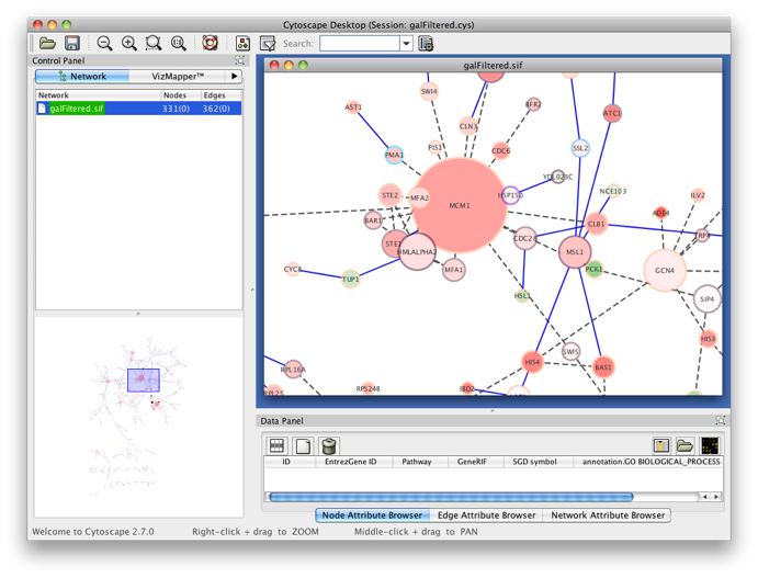
Start Cytoscape and load the network galFiltered.cys from the sampleData folder in the Cytoscape directory. Select PiNGO from the Plugins menu.

Step 2

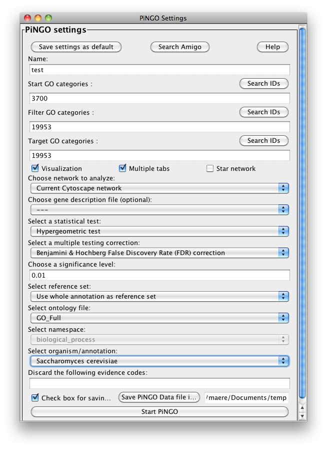
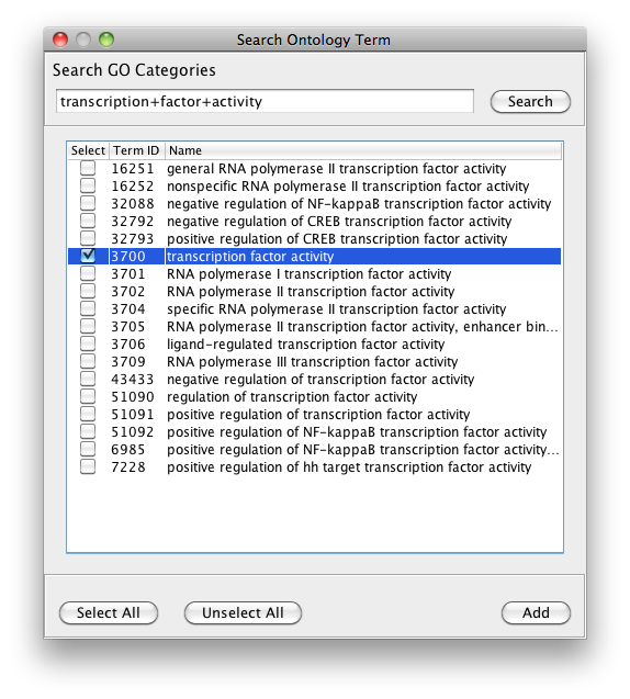
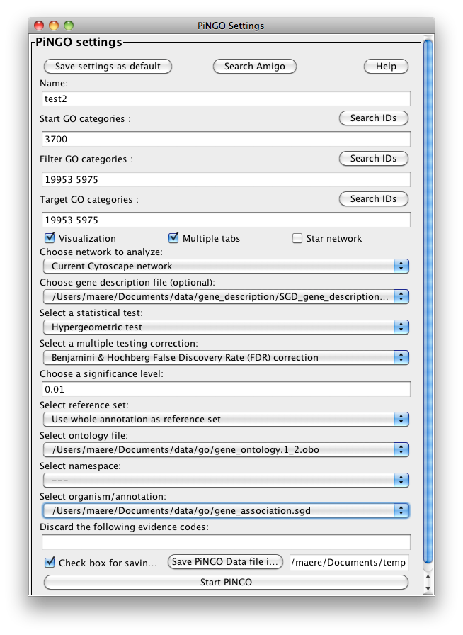
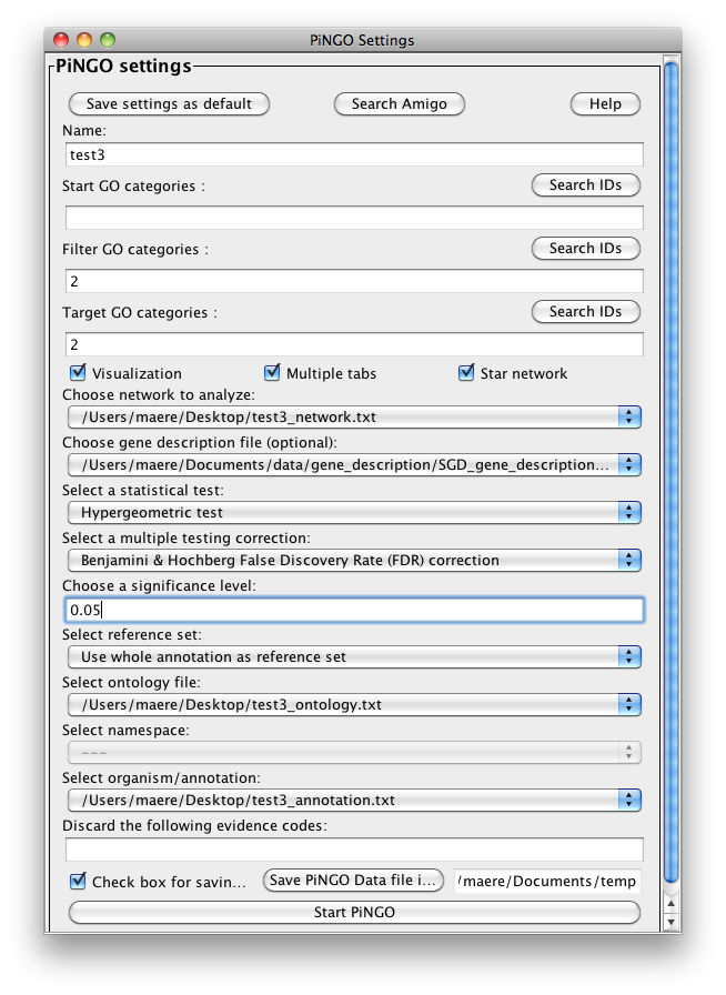
The PiNGO Settings panel pops up. Start by filling in a name for your analysis, e.g. ‘test’. This name will be used for creating the output file and the visualization of the results in Cytoscape. We want to discover transcription factors in the network that might be involved in the process of reproduction in yeast, but that are not yet annotated as such in GO. Select GO_Full from the ontology list under Select ontology file. This choice determines which ontology terms can be used in the GO categories fields. First of all, we will specify which Start GO categories we want to use. Those categories are the classes of genes we want to explore, and in our case transcription factors. Click the Search IDs button next to Start GO categories, and fill in ‘transcription+factor+activity’ in the search dialog (the +’s ensure that the search results will contain all three words, not just 1 or 2). Select ‘transcription factor activity’ from the list using the checkbox at the left, and click the Add button. The GO ID code for the ‘transcription factor activity’ category is transferred to the Start GO categories field. Close the search dialog and click the Search IDs button next to Filter GO categories. Search for ‘sexual+reproduction’ , select the sexual reproduction GO category and transfer it to the Filter GO categories field by clicking the Add button. The text in the the Filter GO categories field should now read ‘19953‘ (sexual reproduction = GO:0019953). Genes already annotated to this category will be filtered out, because we are not interested in discovering known reproduction genes. Finally, fill in 19953 in the Target GO categories field as well (sexual reproduction = GO:0019953). This is the predicted GO annotation we want the candidate genes to have. We want to visualize the results in Cytoscape, so the corresponding box is checked accordingly. The user also has the option of visualizing the results for different Target categories in separate output tabs and output networks. This is controlled by the Multiple tabs checkbox. In our case, it doesn’t matter whether the box is checked or not since we only specified one Target GO category. The third checkbox next to the Multiple tabs checkbox controls the topology of the output network. When Star network is checked, the output networks will only contain edges from candidate genes to neighbors of those genes in the input network (see below) that are annotated to one of the Target GO categories. If Star network is unchecked, connections between the neighbors will also be displayed. Let’s leave it unchecked. Select Current Cytoscape network from the Choose network to analyze dropdown menu. Then select a statistical test (the Hypergeometric Test is exact and equivalent to an exact Fisher test, the Binomial Test is less accurate but quicker) and a multiple testing correction (we recommend Benjamini & Hochberg's FDR correction, the Bonferroni correction will be too conservative in most cases), and choose a significance level, e.g. 0.01. We're interested in assessing the enrichment of functional categories in a gene’s neighborhood with respect to the whole yeast genome, which is why we choose the Whole Annotation as the reference set. We’ve already selected GO_Full from the ontology list, and now we select Saccharomyces cerevisiae from the organism list. Note that it is recommended in most cases to use custom annotation and ontology files instead, see further. We want to consider all GO annotation evidence codes, so don't fill in anything in the evidence code box. Finally, select a directory to save the output file in (the file will be named test.pgo if you filled in test as a descriptive name), and press Start PiNGO...

Step 3

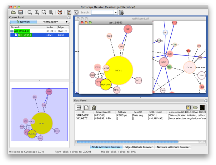
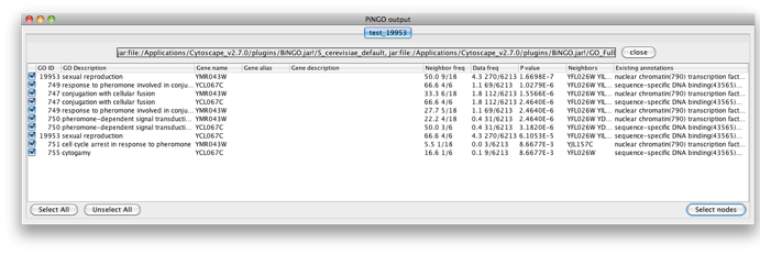
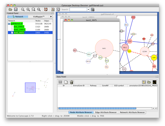
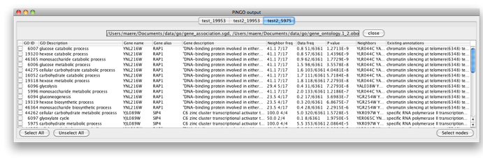
The program will inform you of its progress while parsing the annotations and calculating the tests and layout. Finally, a visualization of the discovered candidate genes is created in Cytoscape. When analyzing an existing Cytoscape network, all discovered candidate genes and neighboring nodes that are annotated to the Target GO category (i.e. the genes that gave rise to the discovery of the candidate gene) are visualized as a subnetwork of the original network. The list of candidate genes, with p-values and original GO annotations is shown in the PiNGO output window. Note that predictions for all subcategories of the target GO categories are also produced. You can sort on the different columns by clicking the header. The same information is stored in the test.pgo output file in the output directory you specified. Congratulations ! You just performed your first PiNGO analysis...

Select some interesting candidate genes by checking the boxes on the left side of the PiNGO output window. Then press the Select nodes button. These nodes will be highlighted in the output Cytoscape network.

Step 4

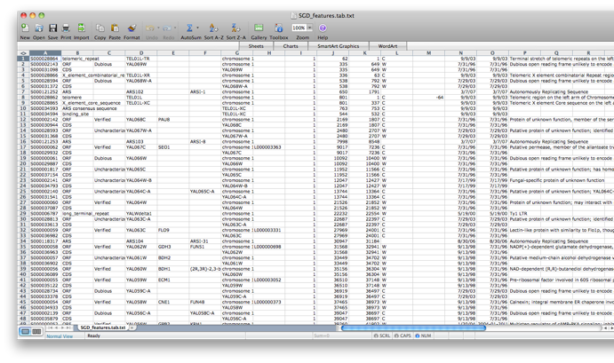
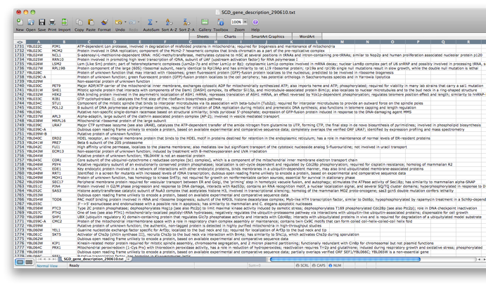
Go back to the network by clicking on the galFiltered.sif in the left panel on the Cytoscape desktop. Go to the PiNGO Settings panel (you do not have to start a new PiNGO session), choose a new name (test2) and adjust some of the settings you made earlier. As an alternative to using the default annotations, you can download up-to-date files from the GO website (www.geneontology.org). Download the most recent gene ontology .obo file (e.g. gene_ontology.1_2.obo) and the gene association file for S. cerevisiae (gene_associations.sgd). Store them somewhere, and select those files under Custom... in the annotation and ontology dropdown boxes of the PiNGO Settings Panel. The namespace panel becomes active. Select ‘---’ which means you want to use the full ontology structure for making predictions, not some subset. Add a category to the target and filter GO categories, e.g. 5975 for carbohydrate metabolism (GO:0005975). If you feel like it, download the file SGD_features.tab from http://www.yeastgenome.org/gene_list.shtml, open it in Excel or some other spreadsheet program, delete all columns except for D, E and P, sort it to get rid of empty lines and save the resulting sheet as a tab-delimited text file (see screen shots below). We will use this file as a gene description file. Select it under the Choose gene description file menu. Press start...

PS If you want to use the same custom files over and over again and want to avoid to each time navigate your directories in search of the proper files, you can save your present settings as default by using the save settings button on the top left of the PiNGO Settings Panel.

Step 5

You will get the following screen. Observe that multiple output networks are created, one per Target GO category that you specified, because we selected the Multiple tabs option. The resulting GO subnetworks will be labeled with the name you set for the analysis and the target GO ID number. Try some other settings and options. In most cases, PiNGO will stop you if you're about to do something wrong. Still, there are several peculiarities and potential pitfalls you should keep in mind while using PiNGO. Please look at the Manual and the FAQ for more details.

Tutorial 2

Step1

Now let’s use a custom network loaded from a file. We’ll use an artificial network with artificial annotation categories and ontology structure, to demonstrate PiNGO’s use on non-GO ontology structures. First make a network file like this (make sure the genes are separated by tabs) and save it as test3_network.txt :

gene1 gene2

gene1 gene3

gene1 gene4

gene1 gene5

gene2 gene3

gene2 gene4

gene2 gene5

gene3 gene4

gene3 gene5

gene4 gene5

gene6 gene7

gene6 gene8

gene6 gene9

gene6 gene10

gene7 gene8

gene7 gene9

gene7 gene10

gene8 gene9

gene8 gene10

gene9 gene10

gene11 gene1

gene11 gene2

gene11 gene3

gene11 gene4

gene11 gene5

gene12 gene6

gene12 gene7

gene12 gene8

gene12 gene9

gene12 gene10

Make a custom ontology file that contains 4 categories (test3_ontology.txt):

(curator=me)(type=custom)

1 = cat1

2 = cat2 [isa: 1 ]

3 = cat3 [isa: 1 ]

4 = cat4 [isa: 3 ]

and an annotation file like this (test3_annotation.txt):

(species=weird)(type=custom)(curator=me)

gene1 = 2

gene2 = 2

gene3 = 2

gene4 = 2

gene5 = 2

gene6 = 4

gene7 = 4

gene8 = 4

gene9 = 4

gene10 = 4

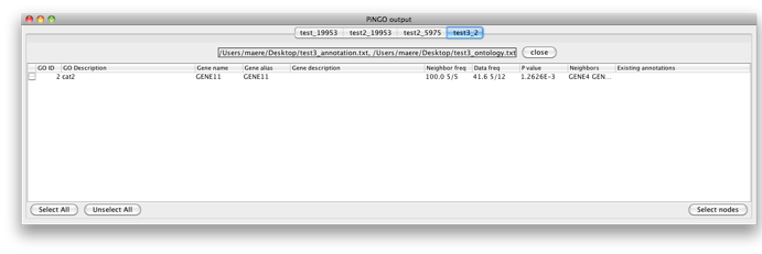
So basically you’ve defined two clusters of 5 nodes that are completely interconnected (nodes 1-5 and 6-10), with different annotations (2 and 4 respectively). Two unknown genes, 11 and 12, are linked to the first and second cluster, respectively. Specify the custom files you just made in the right dropdown boxes under Custom... , and set the other settings as in the figure below. Notice that nothing is specified in the Start categories box, this means that we want to take into account all genes as potential candidates. Press Start...

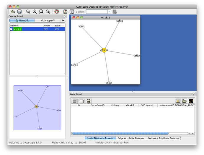
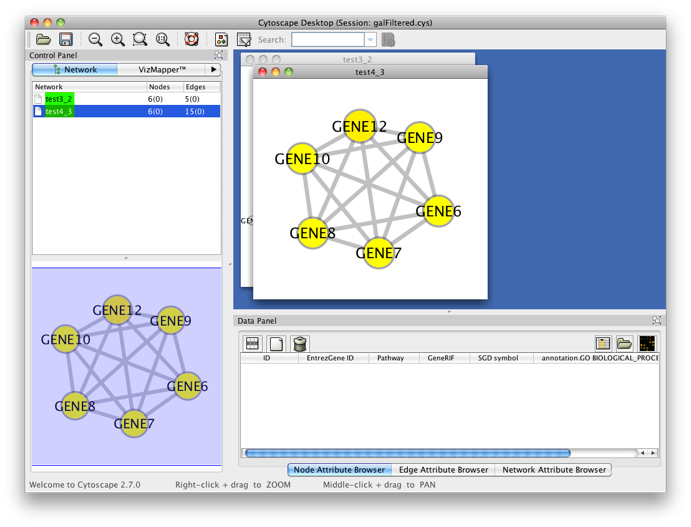
You’ll get the following result. A PiNGO network calculated from custom network files has its own visual style (called PiNGO Style for <network name> in Cytoscape’s Vizmapper), mapping attributes such as p-values and number of genes belonging to the target GO category in the neighborhood of a candidate gene to the color and the size of the nodes, respectively. Uncolored nodes are nodes that are annotated to the Target GO category and that are linked to a newly discovered candidate gene in the original network. Colored nodes represent candidate genes that are predicted to be associated to the target GO category at the chosen significance level. In case multiple p-values are calculated for a given node, e.g. for different target categories or different subcategories of a target category, the color of the node corresponds to the minimum (most significant) p-value obtained. More significant p-values give rise to more orange colored nodes (see also the Color Legend panel). In this case, node 11 is the only candidate gene discovered, as expected. Notice the star topology of the output: we’ve chosen the option Star network which does not display network connections between neighbors of candidate genes. If you'd like another layout, e.g. hierarchical, select the corresponding option from the Cytoscape Visualization menu.

Step 2

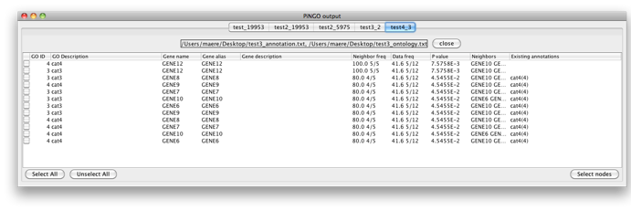
Now fill in 3 as a Target GO category and leave the Start Filter GO category field blank. PiNGO will now consider genes already annotated to category 3 as potential target genes. Press Start... Genes 6-10 are predicted to be part of cat3 and cat4. Note that the whole cluster was originally annotated to cat4 and cat4 is a subcategory of cat3, so all of them are annotated to cat3 as well in the original annotation, since annotations propagate upwards through the hierarchy. However, this has no influence on the results since the annotation of the candidate genes themselves is not taken into account while making predictions. Gene 12 is also predicted to be part of cat4, as expected.